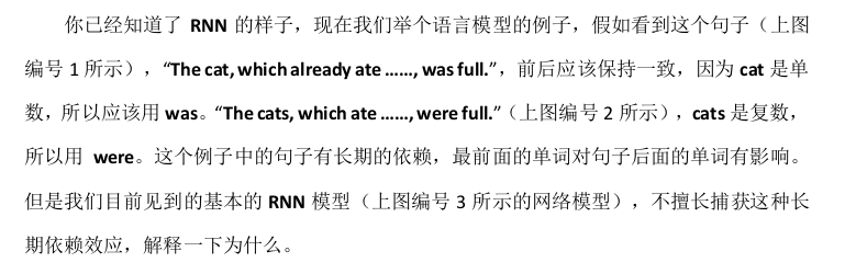
RNN
循环神经网络是从左向右扫描数据,同时每个时间步的参数也是共享的,所以下页幻灯
片中我们会详细讲述它的一套参数,我们用W ax 来表示管理着从x <1> 到隐藏层的连接的一系列参数,每个时间步使用的都是相同的参数W ax 。而激活值也就是水平联系是由参数W aa 决
定的,同时每一个时间步都使用相同的参数W aa ,同样的输出结果由W ya 决定。下图详细讲述
这些参数是如何起作用。
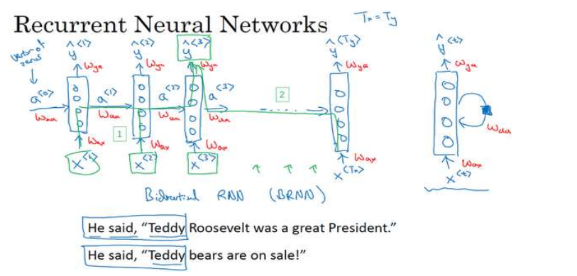
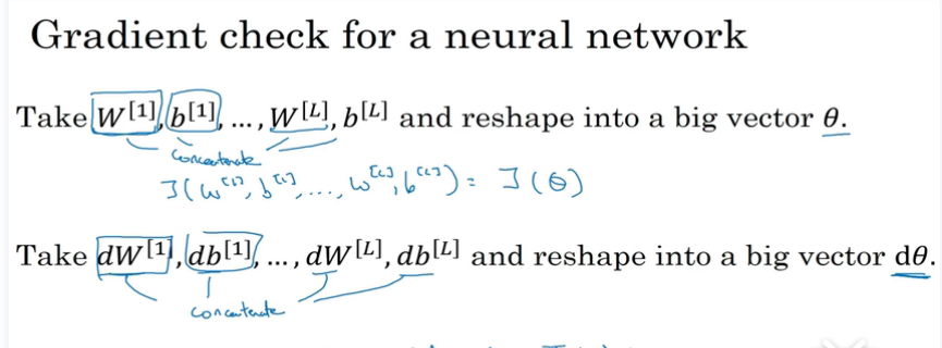
意思是说当预测y^[3]的时候不仅仅需要输入的x^[3]信息,还需要输入的x^[1],x^[2]信息。
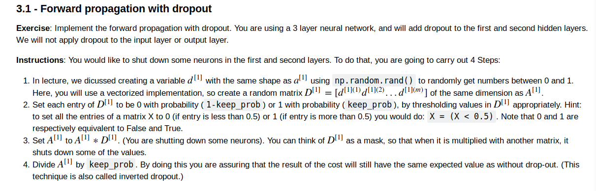
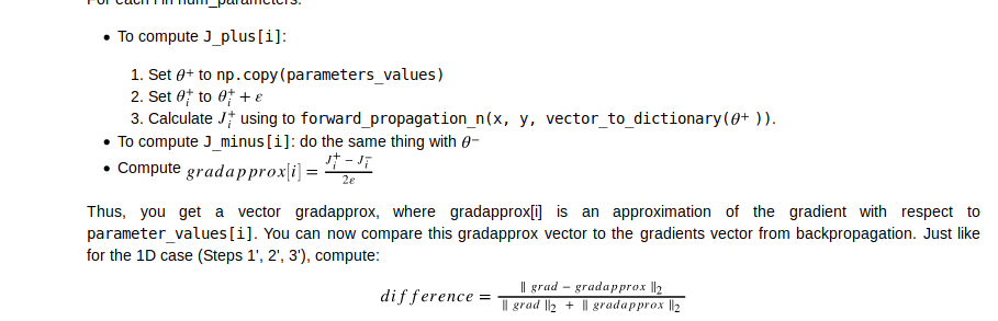
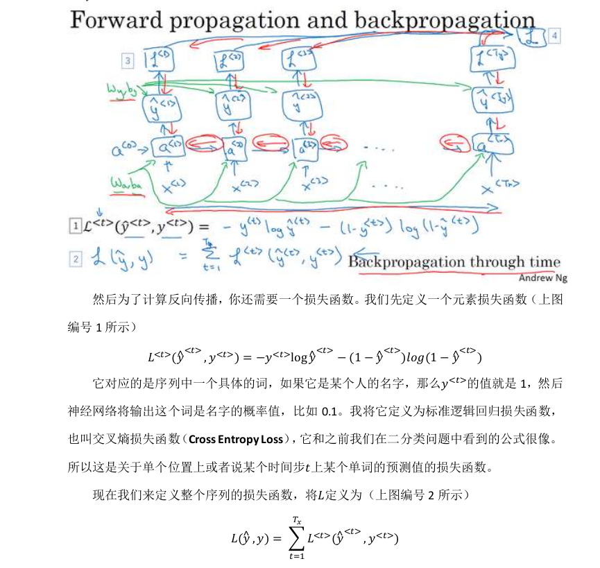
forward propagation
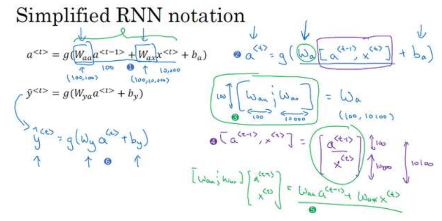
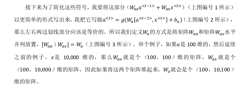
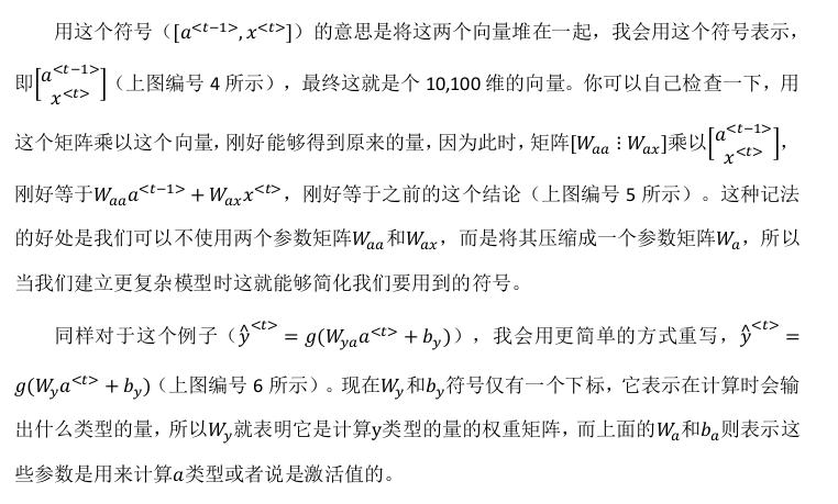
simplification notation
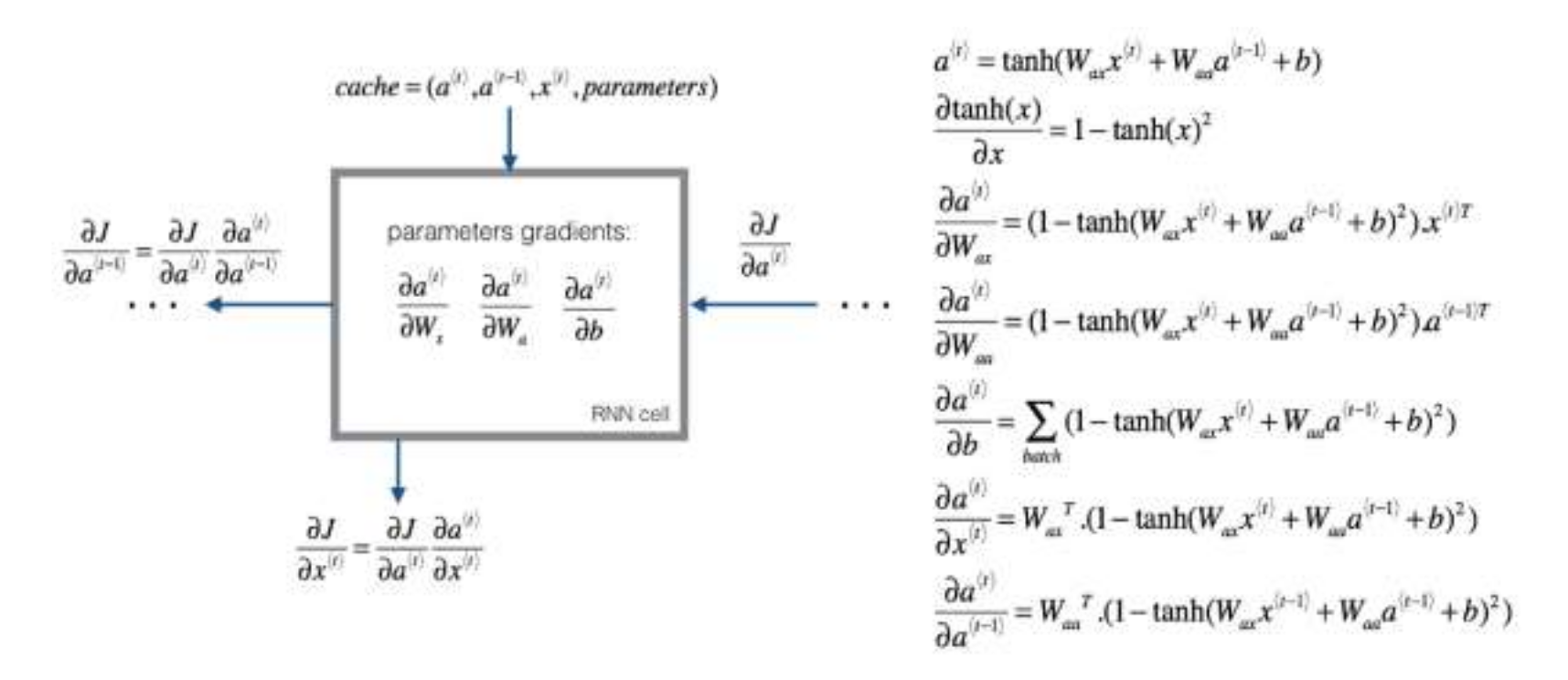
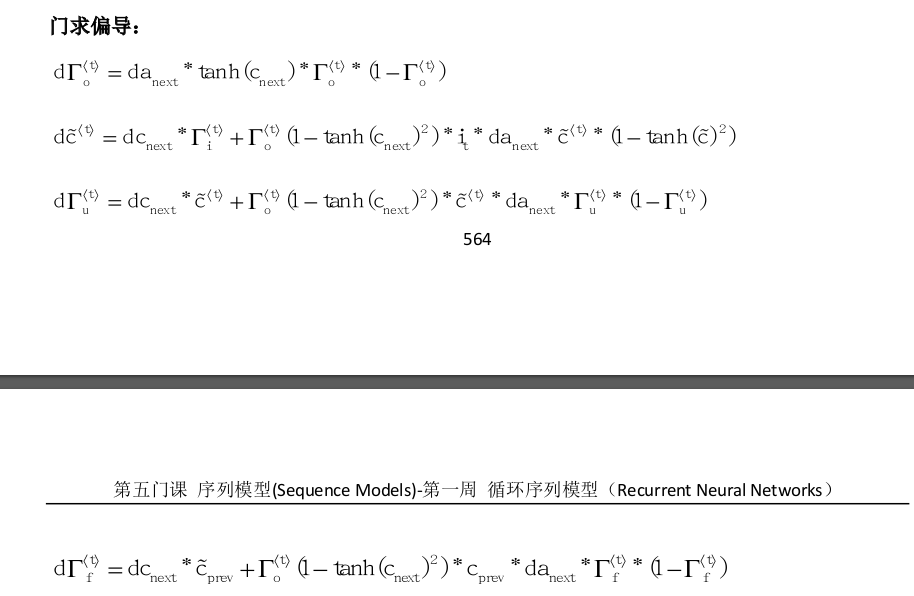
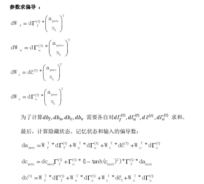
backward propagation
求导示意图:
RNN种类
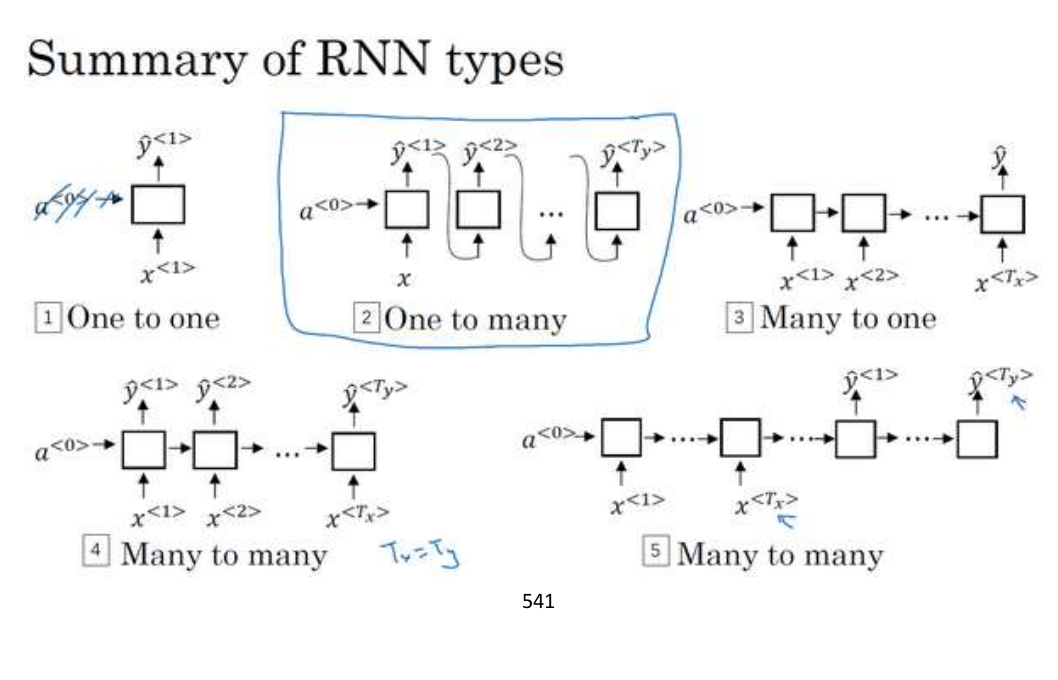
1 to 1
1 to many 音乐生成、序列生成
many to 1 情感判断
many to many 如 name entity recognition
many to many 如 翻译,例如输入的x是中文,输出的y是英文
训练一个语言模型
1
建立一个字典,把输入句子每个单词转化为对应的one-hot向量。
有时候要在句子末尾添加一个EOS标记,表示句子的结束。未知的词用UNK来代替。
2.
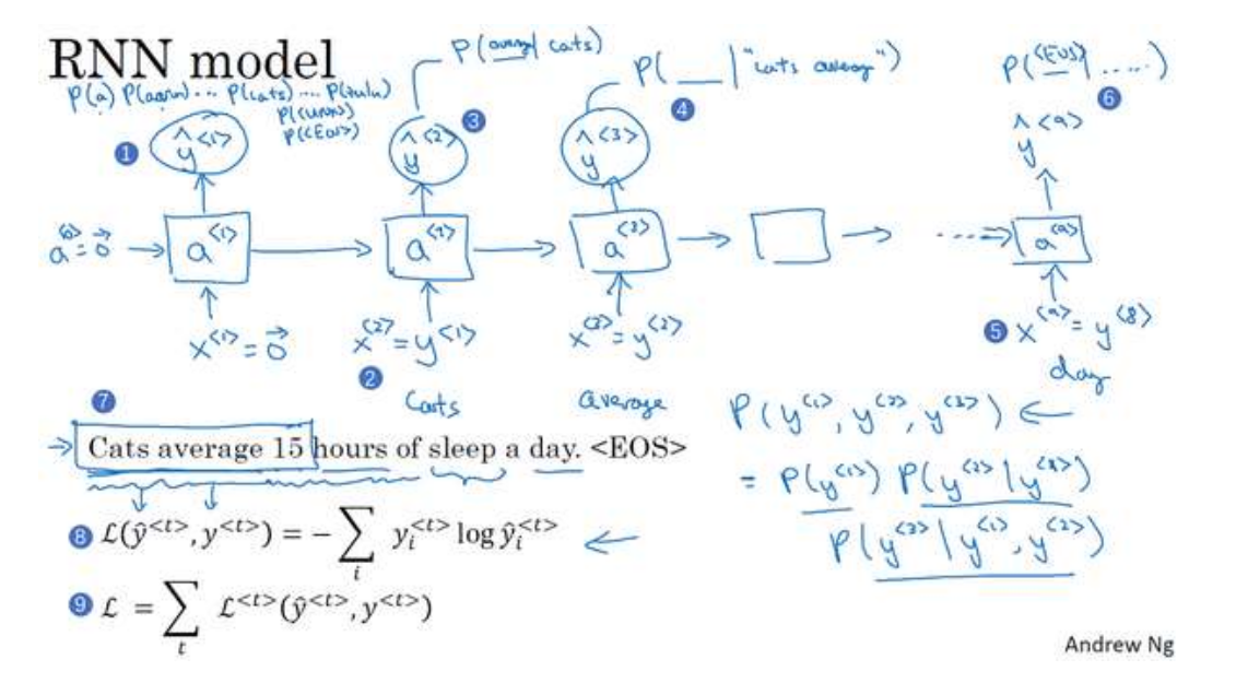
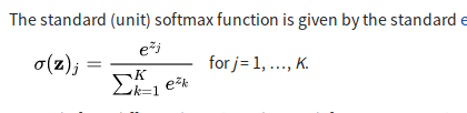
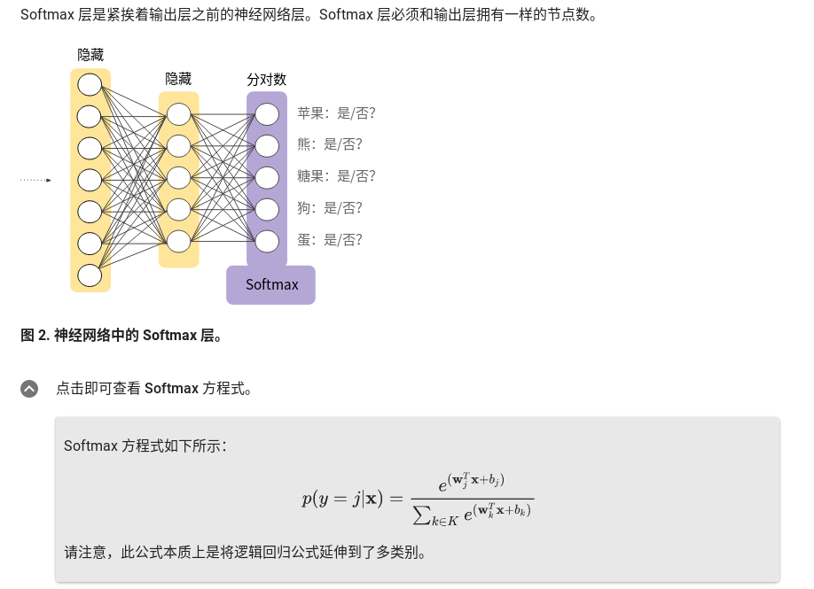
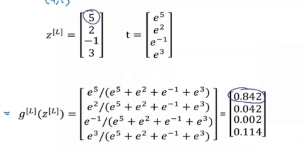
建立RNN模型,x^[1]会被设为一个0向量,在之前的a^[0]也会被设为一个0向量,于是a^[1]要做的是通过softmax进行一些预测来计算第一个词可能会是什么,结果就是y^[1],这一步就是通过一个softmax层来预测字典中任意单词会是第一个词的概率,输出是softmax的计算结果,结果个数就是字典的词的个数。
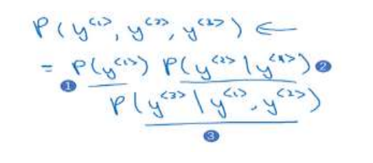
然后预测第二个词:是在考虑预测了第一个词的基础上预测到第二个词的概率。
如此类推,这是一个全概率公式。
把这三个概率相乘,含义就是最后得到这个含3个词的整个句子的概率。
对新序列采样
训练了一个序列模型之后,想要了解这个模型学到了什么,一种非正式方法就是进行一次新序列采样。
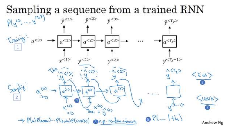
就是如何从RNN语言模型中生成一个随机选择的句子:
第一步要做的就是对你想要模型生成的第一个词进行采样,于是你输入x <1> = 0,
a <0> = 0,现在你的第一个时间步得到的是所有可能的输出是经过 softmax 层后得到的概率,
然后根据这个 softmax 的分布进行随机采样。Softmax 分布给你的信息就是第一个词 a 的概
率是多少,第一个词是 aaron 的概率是多少,第一个词是 zulu 的概率是多少,还有第一个词
是 UNK(未知标识)的概率是多少,这个标识可能代表句子的结尾,然后对这个向量使用例
如 numpy 命令, np.random.choice (上图编号 3 所示),来根据向量中这些概率的分布
进行采样,这样就能对第一个词进行采样了。
然后再到下一个时间步,无论你得到什么样的用 one-hot 码表示的选择结果,都把它传
递到下一个时间步,然后对第三个词进行采样。不管得到什么都把它传递下去,一直这样直
到最后一个时间步。
这就得到了一个随机生成的句子。
基于字符的语言生成模型
对于英文来说,字典仅包含26个英文字母大小写,标点符号等等。
优点:不必担心出现未知的的标识。
缺点:不能像基于词汇的模型,可以捕捉长范围上下文的关系,而且计算成本会很高。
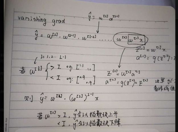
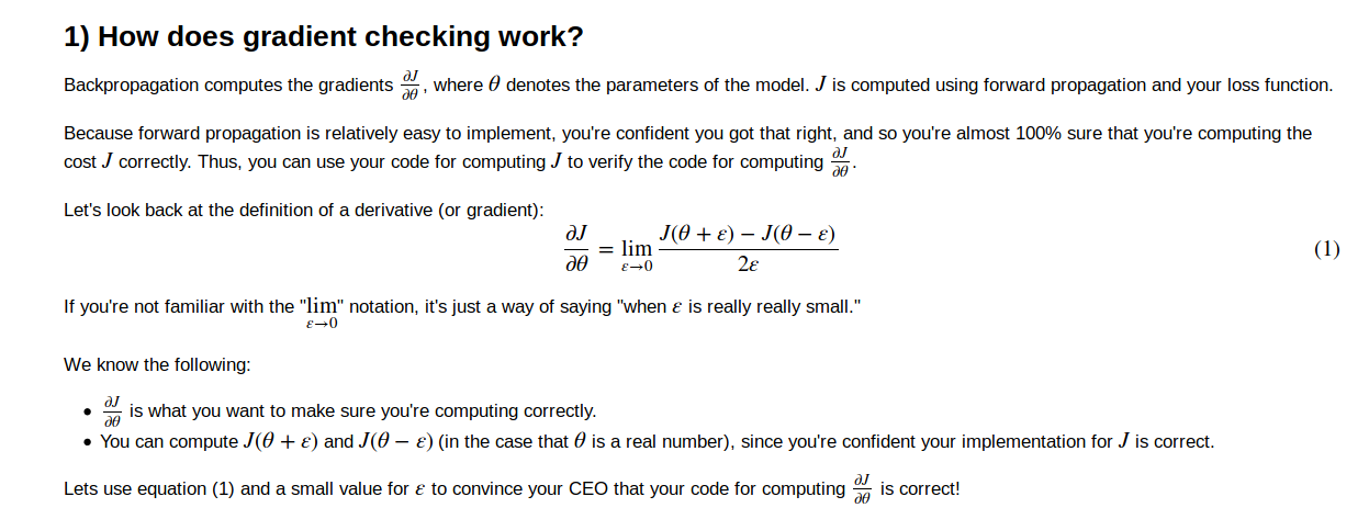
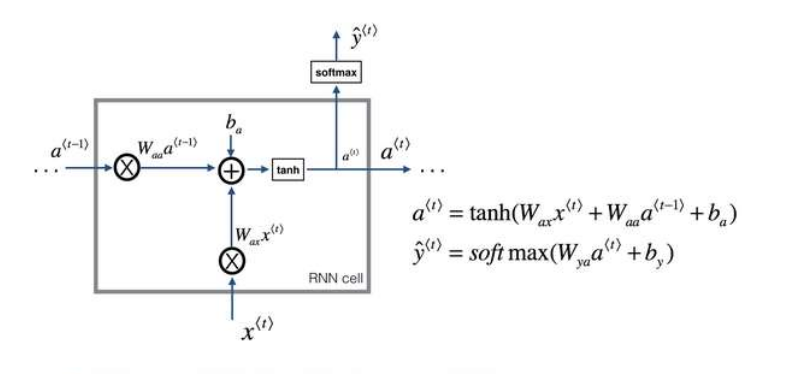
RNN的问题
1.因为梯度消失,不擅长处理长期依赖的问题。
对于 RNN,首先从左到右前向传播,然后反向传播。但是反向传播会很困难,因为同样的梯度消失的问题,后面层的输出误差很难影响前面层的计算,实际上很难让一个神经网络能够意识到他要记住看到的是单数名词还是复数名词。
2.对于梯度爆炸问题则比较好解决。
一个方法是 gradient clipping,意思是观察你的梯度向量,如果它大于某个阈值,则缩放梯度向量,保证他不会太大。
GRU (gated recurrent unit)
门控循环单元
GRU 单元将会有个新的变量称为c,代表细胞(cell),即记忆细胞(下图编号 1 所示)。记忆细胞
的作用是提供了记忆的能力,比如说一只猫是单数还是复数,所以当它看到之后的句子的时
候,它仍能够判断句子的主语是单数还是复数。于是在时间t处,有记忆细胞c
们看的是,GRU 实际上输出了激活值a
要使用不同的符号c和a来表示记忆细胞的值和输出的激活值,即使它们是一样的。我现在使
用这个标记是因为当我们等会说到 LSTMs 的时候,这两个会是不同的值,但是现在对于 GRU,c
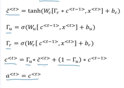
所以这些等式表示了 GRU 单元的计算,在每个时间步,我们将用一个候选值重写记忆
细胞,即c̃
计算, c̃
(下图编号 3 所示)。
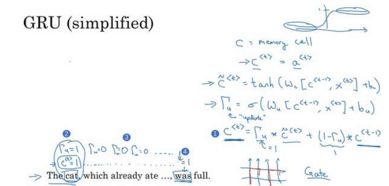
所以我们接下来要给 GRU 用的式子就是c
1 所示)。你应该注意到了,如果这个更新值Γ u = 1,也就是说把这个新值,即c
选值(Γ u = 1时简化上式,c
更新这个值。对于所有在这中间的值,你应该把门的值设为 0,即Γ u = 0,意思就是说不更
新它,就用旧的值。因为如果Γ u = 0,则c
完整的GRU单元
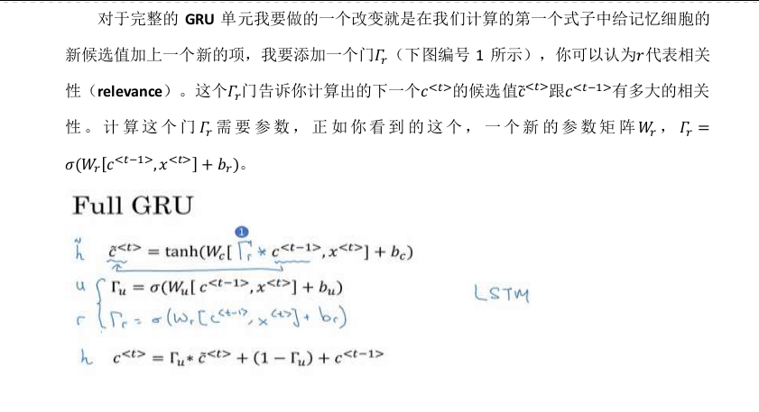
总结:
GRU是用于解决RNN深层网络中梯度弥散问题的一种结构,引入gamma门参数用来决定该时间步的激活层是来自于上一层(保留记忆)还是新计算的结果(不保留记忆)
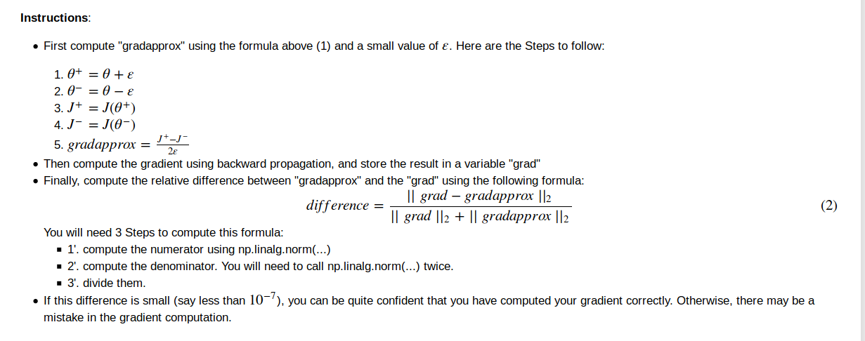
LSTM
回顾GRU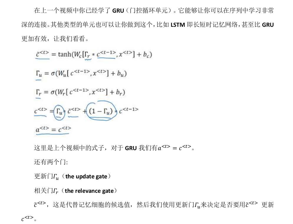
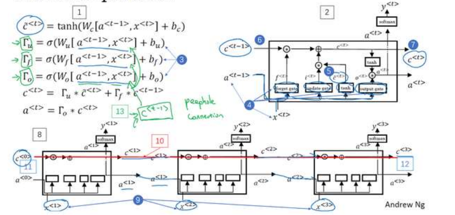
我们像以前那样有一个更新门Γ u 和表示更新的参数W u ,Γ u = σ(W u [a <t−1> , x
然后这里(上图编号 7 所示)用遗忘门(the forget gate),我们叫它Γ f ,所以这个Γ f =
σ(W f [a <t−1> , x
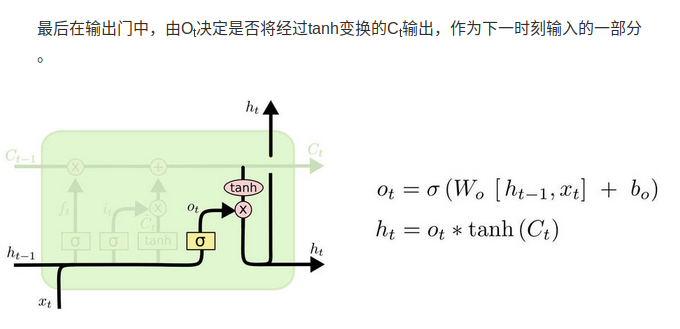
然后我们有一个新的输出门,Γ o = σ(W o [a <t−1> , x
于是记忆细胞的更新值c
所以这给了记忆细胞选择权去维持旧的值c <t−1> 或者就加上新的值c̃
单独的更新门Γ u 和遗忘门Γ f ,然后这个表示更新门(Γ u = σ(W u [a <t−1> , x
遗忘门(Γ f = σ(W f [a <t−1> , x
最后a
peephole connection
门值不仅取决于a <t−1> 和x
这叫做“窥视孔连接”(peephole connection)。虽然不是个好听的名字,但是你想,“偷窥孔
连接”其实意思就是门值不仅取决于a <t−1> 和x
然后“偷窥孔连接”就可以结合这三个门(Γ u 、Γ f 、Γ o )来计算了
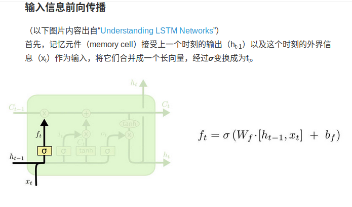
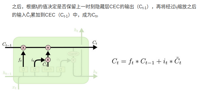
详情可见 http://colah.github.io/posts/2015-08-Understanding-LSTMs/
forward propagate
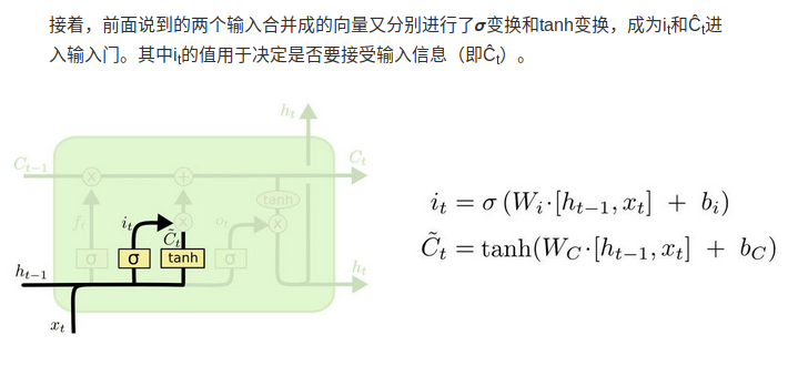
这里的i_t就是update gate,f_t就是forget gate
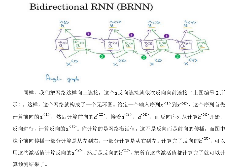
BRNN
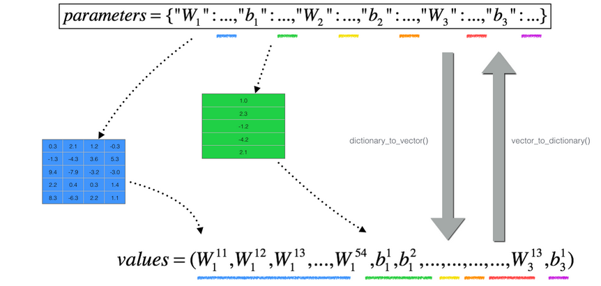
Deep RNN
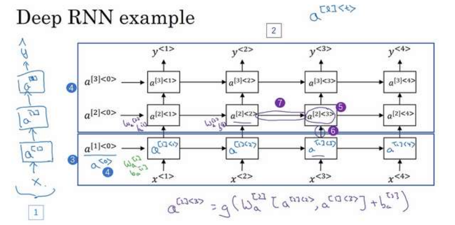
不再用原来的a <0> 表示 0 时刻的激活值了,而是用a [1]<0> 来表示第一层
(上图编号 4 所示),所以我们现在用a [l]
间点,这样就可以表示。第一层第一个时间点的激活值a [1]<1> ,这(a [1]<2> )就是第一层第
二个时间点的激活值,a [1]<3> 和a [1]<4> 。然后我们把这些(上图编号 4 方框内所示的部分)
堆叠在上面,这就是一个有三个隐层的新的网络。
我们看个具体的例子,看看这个值(a [2]<3> ,上图编号 5 所示)是怎么算的。激活值
a [2]<3> 有两个输入,一个是从下面过来的输入(上图编号 6 所示),还有一个是从左边过来
[2]
[2]
的输入(上图编号 7 所示),a [2]<3> = g(W a [a [2]<2> , a [1]<3> ] + b a ),这就是这个激活值的计算方法。参数W a 和b a 在这一层的计算里都一样,相对应地第一层也有自己的参数W a[1]
和b a 。