Train/dev/test sets
dev sets,also called hold-out sets, are used to decide the model’s performance.(give you an unbiased estimate of your model’s performance)
example:
If you have 10,000,000 examples, how would you split the train/dev/test set?
98% train . 1% dev . 1% test
The dev and test set should:
Come from the same distribution
Bias and Variance
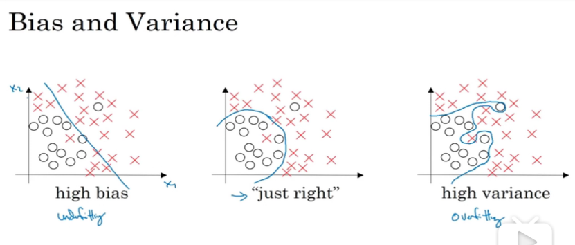
underfitting -> high bias
overfitting -> high variance
example
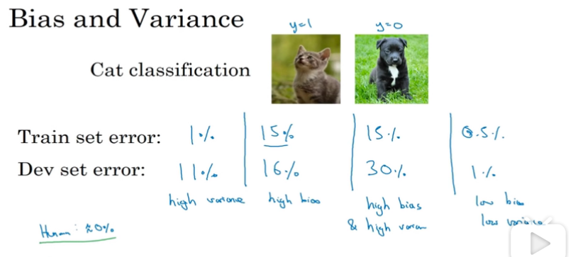
1.如果train error =1%,dev set error = 11%
则overfitting,说明是high variance
2.如果 train error都很大的话,说明是high bias
3.总的来说,如果dev set error 比train set error
大很多,可以说明是overfitting
high bias and high variance
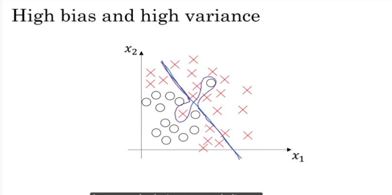
部分数据过拟合,部分欠拟合
basic recipe for ML
如果high bias咋办
High bias (欠拟合)
(training data performance)
- 1.bigger network
- 2.optimized neural network architecture
- 3.other optimizing techniques
High Variance? (过拟合)
(dev data performance)
- 1.more data
- 2.regularization
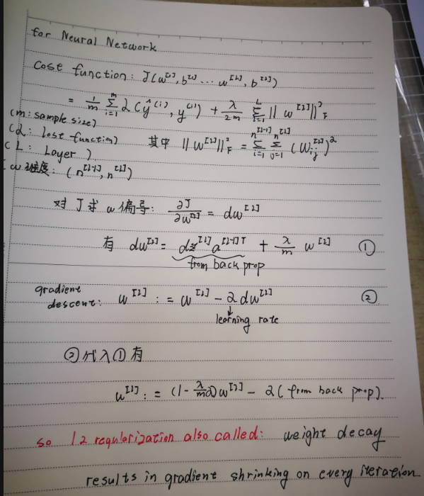
Regularization
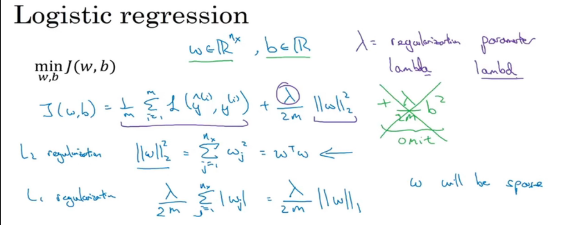
在L1正则化中,w会是一个很sparse的向量,通常在实际应用中L2正则化会应用的更为广泛。
λ 又叫正则化参数
推导
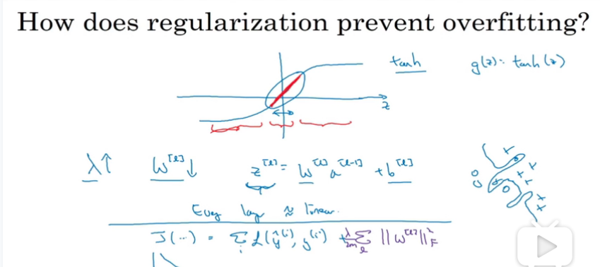
how does it work?
由上面推导我们可知,如果λ越大,那么w会越接近于0,那么以下图的激活函数为例,如果z很小的时候,tanh结果会接近于线性的,,神经网络每一层都将近似于一个线性神经元,那么就可以有效解决过拟合问题,往”欠拟合”或者刚好的方向。
drop out
let’s say a nn with layer l = 3,keep_prob = 0.8
1 | d3= np.random.rand(a3.shape[0],a3.shape[1])<keep_prob |
80%的unit会被保留,20%会被drop out
上面语句作用是d380%元素为1,20%元素为0
1 | a3 = np.multiply(a3,d3) |
然后再scale up
1 | a3/= keep_prob |
why does it work?
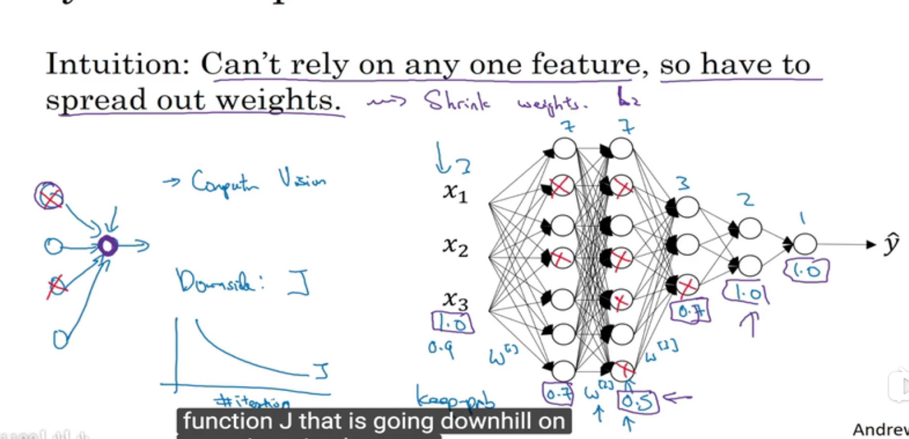
1.在一些神经元很多的层,设置keep_probs低一点,可以有效减少过拟合,实际上是减弱regularization 的作用,在一些神经元很少的层,设置为1.0就好
2.在CV领域,由于输入数据的维数通常很大,一般都需要drop out
3.但是drop out会导致不能够通过画出cost function曲线来debug,解决方法是最开始先把所有keep_prob set to 1,then if no bug, turn on drop out
other technique of reducing overfitting
early stopping
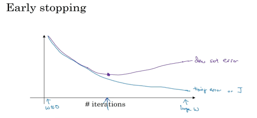
防止dev set error增加,采取early stopping,最后会得到一个middle-size的||w||^2
data augmentation
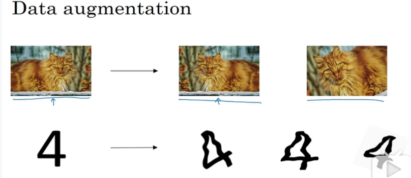
通过变换现有的数据集,来获得更多的数据集
normalizing inputs
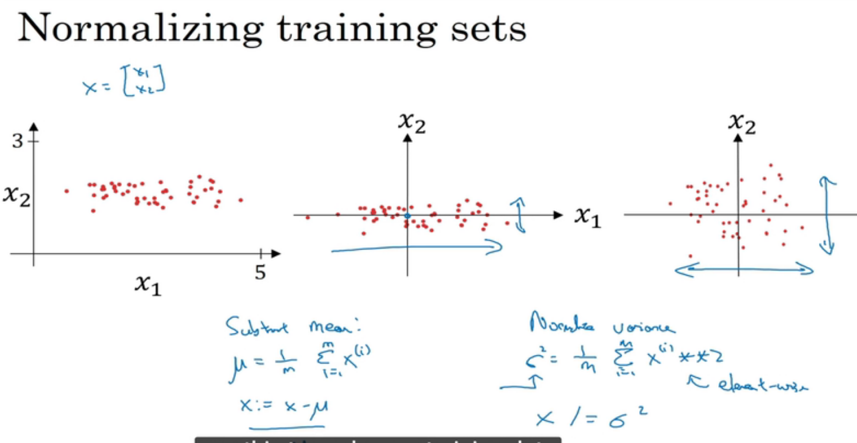
by subtract the mean and scalling the variance
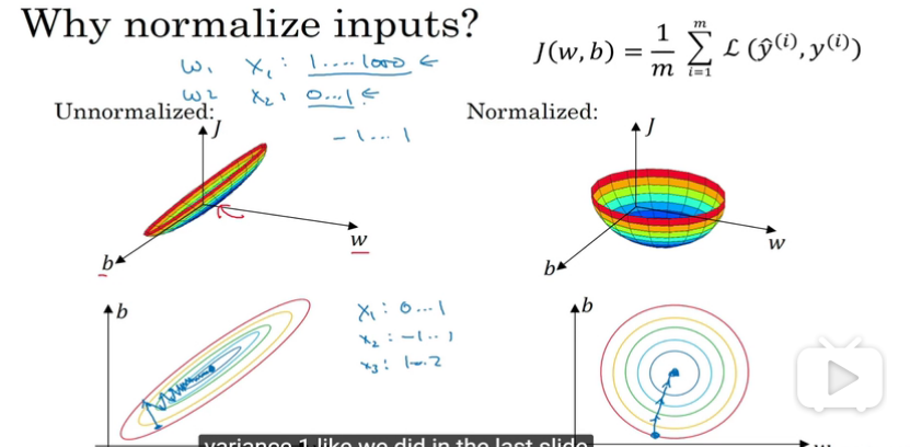
效果就是会加快optimizing 的速度
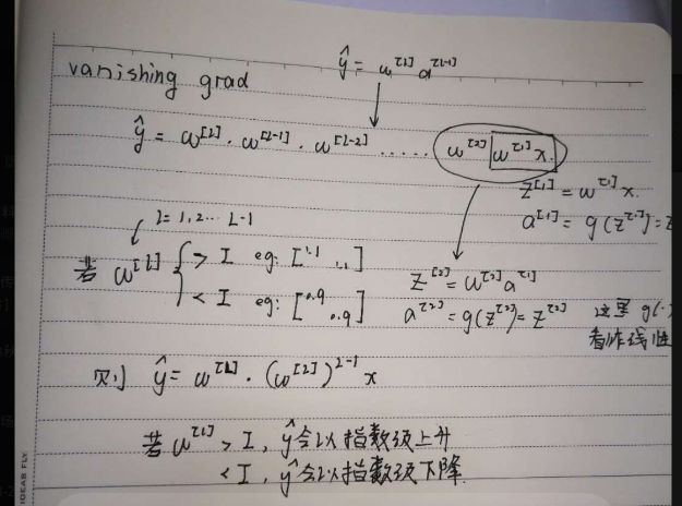
Vanishing gradients
很深层的神经网络,权重相乘累积起来的话后果很严重
参数初始化方法:
这样可以使得w的值接近于1,不会导致梯度消失和梯度爆炸
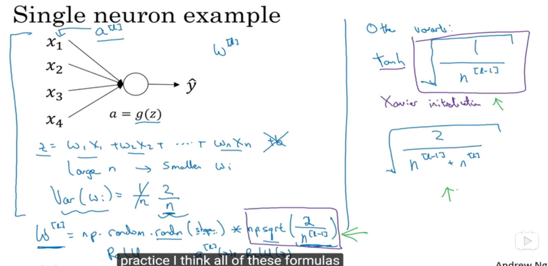
其中的Xavior initialization
可以用来保证输入输出数据的分布相近,加快收敛速度(方差与均值大概相同)
https://blog.csdn.net/shuzfan/article/details/51338178
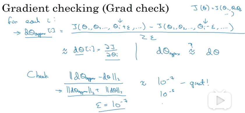
gradient checking
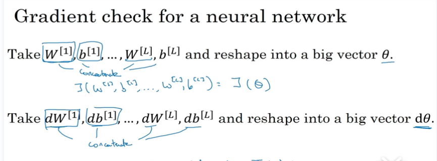
grad check
notes
1.no use in training ,only to debug
2.if fails grad check,look at components to try to identify bug.
3.remember regularization
4.doesn’t work with dropout
5.run at random initialization
initialization
zero initialization
如果把W矩阵初始化为0的话,相当于在训练一个各层只有一个神经元的神经网络,因为每一层的每个神经元其实都在学习相同的参数。
这时候神经网络只相当于一个线性分类器。
但是bias可以设置处值为0
large random initialization
1.poor initialization can lead to vanishing/exploding gradients
2.如果一开始w初值非常大,梯度下降所花时间会很长,(需要更多迭代次数)
He random initialization
1 | def initialize_parameters_he(layers_dims): |
xavier random initialization
只是把 sqrt(2./layers_dims[l-1]) 换作sqrt(1./layers_dims[l-1])
L2 Regularization
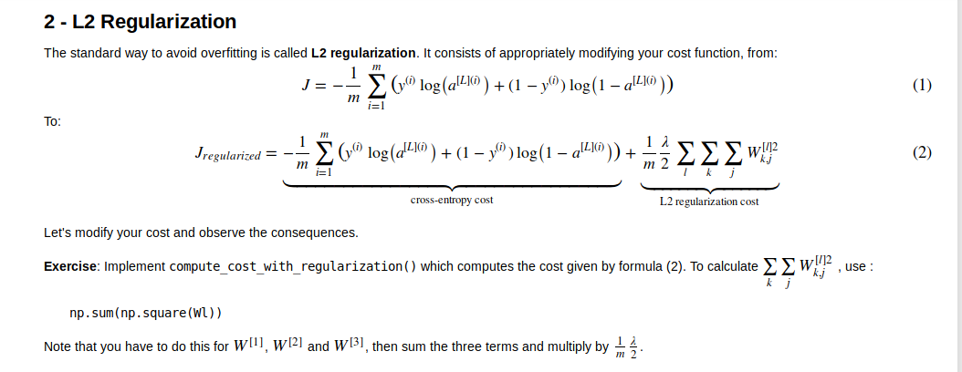
同时code如下
1 | def compute_cost_with_regularization(A3, Y, parameters, lambd): |
同时引入正则化的话,在backword propa的时候,要加上正则项

code1
2
3
4
5
6
7
8
9
10
11
12
13
14
15
16
17
18
19
20
21
22
23
24
25
26
27
28
29
30
31
32
33
34
35
36
37
38
39
40
41
42
43def backward_propagation_with_regularization(X, Y, cache, lambd):
"""
Implements the backward propagation of our baseline model to which we added an L2 regularization.
Arguments:
X -- input dataset, of shape (input size, number of examples)
Y -- "true" labels vector, of shape (output size, number of examples)
cache -- cache output from forward_propagation()
lambd -- regularization hyperparameter, scalar
Returns:
gradients -- A dictionary with the gradients with respect to each parameter, activation and pre-activation variables
"""
m = X.shape[1]
(Z1, A1, W1, b1, Z2, A2, W2, b2, Z3, A3, W3, b3) = cache
dZ3 = A3 - Y
### START CODE HERE ### (approx. 1 line)
dW3 = 1./m * np.dot(dZ3, A2.T) + (lambd/m)*W3
### END CODE HERE ###
db3 = 1./m * np.sum(dZ3, axis=1, keepdims = True)
dA2 = np.dot(W3.T, dZ3)
dZ2 = np.multiply(dA2, np.int64(A2 > 0))
### START CODE HERE ### (approx. 1 line)
dW2 = 1./m * np.dot(dZ2, A1.T) + (lambd/m)*W2
### END CODE HERE ###
db2 = 1./m * np.sum(dZ2, axis=1, keepdims = True)
dA1 = np.dot(W2.T, dZ2)
dZ1 = np.multiply(dA1, np.int64(A1 > 0))
### START CODE HERE ### (approx. 1 line)
dW1 = 1./m * np.dot(dZ1, X.T) + (lambd/m)*W1
### END CODE HERE ###
db1 = 1./m * np.sum(dZ1, axis=1, keepdims = True)
gradients = {"dZ3": dZ3, "dW3": dW3, "db3": db3,"dA2": dA2,
"dZ2": dZ2, "dW2": dW2, "db2": db2, "dA1": dA1,
"dZ1": dZ1, "dW1": dW1, "db1": db1}
return gradients
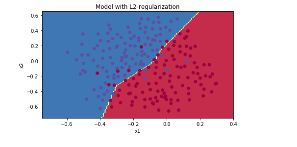
lambd = 0.6
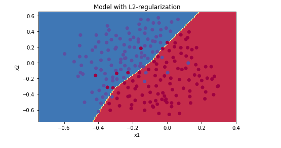
lambd = 0.7
lambd = 0.8
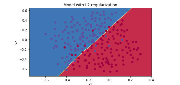
λ增大,能够减少过拟合现象,但是training set error 也会随之减少
drop out
what is inverted dropout?
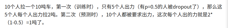
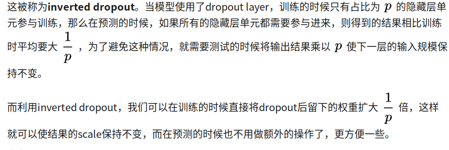
drop out
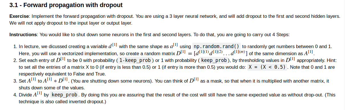
1.创建一个np.array D1 which has the same size as A1(np.random.randn(A.shape[0],A.shape[1]))
2.当A的元素<D[keep_prob]的时候为1,大于的时候为0
3.A = np.multiply(A,D)
4.scale A,i.e. A/=keep_prob (inverted dropout)
1 | def forward_propagation_with_dropout(X, parameters, keep_prob=0.5): |
drop out in backward
just perform dA2*=D2 and scaling
1 | def backward_propagation_with_dropout(X, Y, cache, keep_prob): |
gradient checking
以J = x*theta 为例
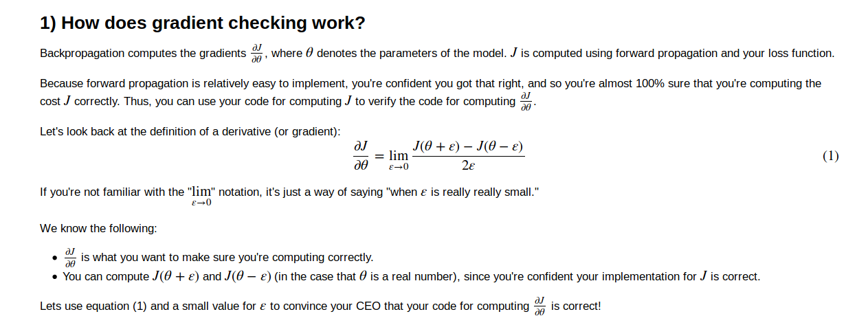
implementation
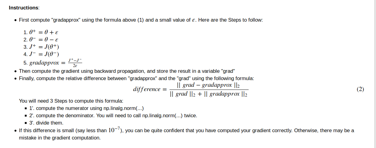
注意1
np.linalg.norm 是求范数的函数,默认是求二范数
1 | def gradient_check(x, theta, epsilon = 1e-7): |
对于多维的情况
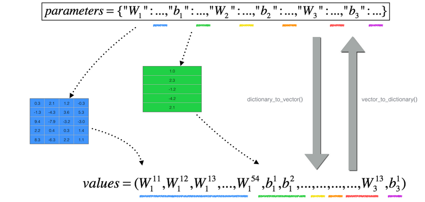
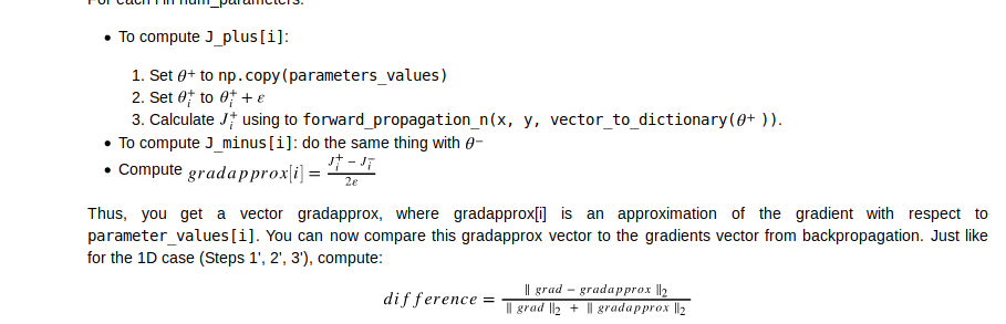
把所有params压缩到一个向量,然后一个for循环,计算每个参数的grad,gradapprox,并加入到一个向量当中,分别得到一个gradapprox与grad向量,再利用这两个向量求范数,求difference
code1
2
3
4
5
6
7
8
9
10
11
12
13
14
15
16
17
18
19
20
21
22
23
24
25
26
27
28
29
30
31
32
33
34
35
36
37
38
39
40
41
42
43
44
45
46
47
48
49
50
51
52
53
54
55
56
57
58
59
60
def gradient_check_n(parameters, gradients, X, Y, epsilon=1e-7):
    """
    Checks if backward_propagation_n computes correctly the gradient of the cost output by forward_propagation_n

    Arguments:
    parameters -- python dictionary containing your parameters "W1", "b1", "W2", "b2", "W3", "b3":
    grad -- output of backward_propagation_n, contains gradients of the cost with respect to the parameters.
    x -- input datapoint, of shape (input size, 1)
    y -- true "label"
    epsilon -- tiny shift to the input to compute approximated gradient with formula(1)

    Returns:
    difference -- difference (2) between the approximated gradient and the backward propagation gradient
    """

    # Set-up variables
    parameters_values, _ = dictionary_to_vector(parameters)
    grad = gradients_to_vector(gradients)
    num_parameters = parameters_values.shape[0]
    J_plus = np.zeros((num_parameters, 1))
    J_minus = np.zeros((num_parameters, 1))
    gradapprox = np.zeros((num_parameters, 1))

    # Compute gradapprox
    for i in range(num_parameters):

        # Compute J_plus[i]. Inputs: "parameters_values, epsilon". Output = "J_plus[i]".
        # "_" is used because the function you have to outputs two parameters but we only care about the first one
        ### START CODE HERE ### (approx. 3 lines)
        thetaplus =  np.copy(parameters_values)                                       # Step 1
        thetaplus[i][0] = thetaplus[i][0] + epsilon                                   # Step 2
        J_plus[i], _ =  forward_propagation_n(X, Y, vector_to_dictionary(thetaplus))  # Step 3
        ### END CODE HERE ###

        # Compute J_minus[i]. Inputs: "parameters_values, epsilon". Output = "J_minus[i]".
        ### START CODE HERE ### (approx. 3 lines)
        thetaminus = np.copy(parameters_values)                                       # Step 1
        thetaminus[i][0] = thetaminus[i][0] - epsilon                                 # Step 2
        J_minus[i], _ = forward_propagation_n(X, Y, vector_to_dictionary(thetaminus)) # Step 3
        ### END CODE HERE ###

        # Compute gradapprox[i]
        ### START CODE HERE ### (approx. 1 line)
        gradapprox[i] = (J_plus[i] - J_minus[i]) / (2 * epsilon)
        ### END CODE HERE ###

    # Compare gradapprox to backward propagation gradients by computing difference.
    ### START CODE HERE ### (approx. 1 line)
    numerator = np.linalg.norm(grad - gradapprox)                                     # Step 1'
    denominator = np.linalg.norm(grad) + np.linalg.norm(gradapprox)                   # Step 2'
    difference = numerator / denominator                                              # Step 3'
    ### END CODE HERE ###

    if difference > 1e-7:
        print("\033[93m" + "There is a mistake in the backward propagation! difference = " + str(difference) + "\033[0m")
    else:
        print("\033[92m" + "Your backward propagation works perfectly fine! difference = " + str(difference) + "\033[0m")

    return difference
concolusion
1.L2正则化和drop out都可以帮你解决overfitting
2.regularization 会使得weight变得非常小